Important note: There exists an un-merged branch tickets/DM-3704
of ip_diffim and pipe_tasks which implements tickets
DM-3704,
DM-5294 and
DM-5295, a refactor of
the large and sprawling code in the existing command-line
tasklsst.pipe.tasks.imageDifference.py. At the time of this
writing, the responsibilities of the existing task were split into two
separate command-line tasks (and their corresponding pipe tasks) and
moved from pipe_tasks into ip_diffim. These new tasks are in the
submodules lsst.ip.diffim.makeDiffim and
lsst.ip.diffim.processDiffim. Correspondingly,
imageDifference.py is now primarily a wrapper around these two tasks
which call MakeDiffimTask.run() and ProcessDiffimTask.run() in
order, taking the same exact input and producing the same exact output
as previously.
The remaining text below will assume that this refactor eventually gets
merged into master, and thus will refer to makeDiffim,
processDiffim, etc.
1. Alard and Lupton (AL) PSF matching and image subtraction
The AL algorithm is used by default in ip_diffim to perform PSF
matching and image subtraction. It performs quickly and well because it
uses small regions surrounding bright, isolated stars around to compute
the PSF-matching kernel, \(k_i\), at various locations \(i\)
across the image. It uses various heuristics to pre-filter those bright
stars prior to computation of the \(k_i\), and once they are
computed, uses PCA to estimate a smoothly spatially-varying \(k\)
from them.
There are a very large number of configuration parameters which affect
the quality of the subtraction. In general, the defaults work well,
although for images with different pixel-scales and/or PSF sizes, these
parameters may need to be tuned. Many of these important parameters are
buried deep in the kernel config parameter of the
lsst.ip.diffim.ImagePsfMatchTask task (which is the subtract
subtask of MakeDiffimTask).
In Figure 1 and Figure 2, we show an
image subtraction using the AL algorithm on an example DECam image. Here
we use a single calexp as the template to highlight the effects of
noise in the template and how these are mitigated. Note that the
subtraction is decorrelated (see Section 1.2.), as this is now the
default when image subtraction is run via the LSST stack.
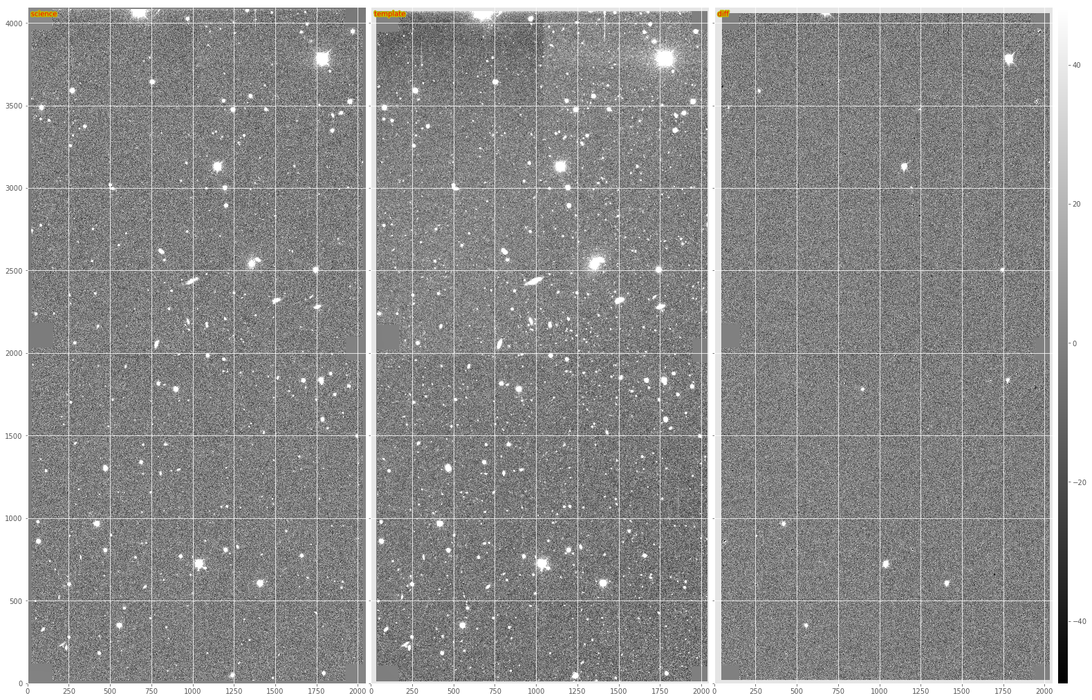
Figure 1 From left to right, sample science image, warped and PSF-matched template, and AL difference image.
Timing: The baseline benchmark for performing basic AL on the example DECam exposure (on my 2015 Macbook 15 with a 2.5 GHz Intel Core i7 is 31.8 seconds. This includes registration and selection of PSF-matching stars, as well as generation of output image files, but excludes any diaSource detection or measurement.
1.1. Pre-convolution
An un-published modification to the AL algorithm was implemented, which accounts for the occasions when the width of the PSF of the science image is \(\leq\) the width of the PSF of the template image. In this case, AL cannot convolve the template to match that of the science image; it instead would need to deconvolve the template, which would result in ringing artifacts. Instead, the science image is “pre-convolved,” or “pre-filtered” with its own PSF, or a Gaussian approximation of it. If the template PSF is narrower than \(\sqrt{2}\times\) that of the science image, then AL will now work, but the resulting image subtraction will have been pre-filtered by the science image’s PSF. This image then corresponds to the match-filtered “likelihood” image subtraction, which has already been convolved with its own PSF, and thus for detection, just needs to be thresholded. A special case is then needed to do any kind of measurement on detected sources in this image. I am not entirely sure how that works.
Timing: Image subtraction with pre-convolution extends the run-time of basic AL from the aforementioned 31.8 seconds to 55.6 seconds, an increase in run-time of \(\sim 75\%\). This is likely due to the need to increase the dimensions of the convolution kernels and stamps upon which PSF matching is performed to ensure that the larger PSF of the pre-convolved science exposure is fully included. Plus the extra convolution, which takes \(\sim 10\) seconds on my machine on the single DECam CCD exposure.
1.2. AL Decorrelation
When the template exposure has significant noise (i.e., is not
constructed from a number of coadds), then AL will correlate the noise
among neighboring pixels when it convolves the template with the
PSF-matching kernel, \(k\). As a result, the noise will be
correlated in the image subtraction, leading to inaccurate detection and
measurement (see DMTN-006 for details).
In DMTN-021, we describe a method for
“decorrelating” the AL image subtraction, and this has been implemented
in the LSST image subtraction code, in the module
lsst.ip.diffim.imageDecorrelation. Decorrelation is toggled via the
doDecorrelation config option, which is enabled by default. Below in
Figure 2 we show a subsection of the images from Figure
1, including both the regular (non-decorrelated) and the
default (decorrelated) AL subtractions on the bottom.
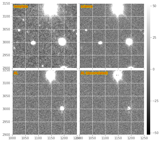
Figure 2 Subsections of a DECam image subtraction, including warped and PSF-matched template, science image, and both decorrelated and non-decorrelated AL difference images.
There occasionally is a problem with decorrelation that I have not been able to narrow down. This problem manifests as noise with a periodic pattern, apparently an overestimated noise problem with some aliasing. This issue is rather rare and I have seen it particularly on notably noisy or poorly reduced images. I believe it is related to the shape/structure of the PSF matching kernel. If the term in the denominator of the expression for \(\psi(k)\) is too close to zero, it will lead to large values in the kernel, which could lead to strange aliasing artifacts in the resulting decorrelated diffim.
See section (1.2.1) below for details and complications of implementing decorrelation in the case of pre-convolution (section 1.1), and see section (3) below for details about how the decorrelation is performed, when accounting for spatially-varying PSFs and noise.
Timing: Enabling decorrelation increases the run-time of the AL algorithm on a sample DECam exposure by \(\sim 10.5\) seconds, or about 33%.
1.2.1. Decorrelation + pre-convolution
The variant of the expression for performing decorrelation in the case of pre-convolution (described above) is given by the deconvolution kernel, \(\psi(k)\) as described in Equation 3 in DMTN-021. The expression includes the pre-filter kernel, \(M(k)\) described above.
This modified decorrelation kernel has been implemented in
ip_diffim, and is used automatically in imageDifference.py when
both the makeDiffim.doDecorrelation and the
makeDiffim.doPreConvolution config options are enabled. In Figure
3, we show the same DECam image subsection as in Figure
2, but in which the template and science image were
swapped and pre-convolution is turned on. The bottom two sub-images show
the resulting match-filtered subtractions, with and without
decorrelation enabled. In many cases the decorrelation kernel is
unstable due to the inclusion of the PSF in the denominator. This leads
to strange aliasing-type artifacts in the resulting decorrelated
likelihood image subtraction, which are extremely large and globally
affect the pixel statistics of the decorrelated, pre-filtered image
subtraction (i.e., give them very large variances). This effect has been
decreased by setting all pixels that are \(\leq 10^{-3}\) to
\(10^{-3}\) in the PSF prior to FFT-ing, but the effect still
remains. Artifacts around bright stars/poorly-subtracted objects are
amplified, and will be difficult to model (visible in Figure
3). This could be mitigated somewhat by better pixel
flagging.
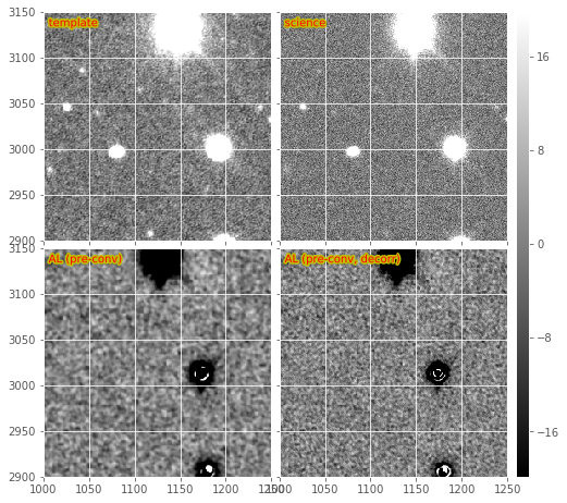
Figure 3 Subsections of a pre-convolved DECam image subtraction, including warped and PSF-matched template, science image, and both decorrelated and non-decorrelated match-filtered AL difference images.
It should also be noted that currently the spatially-varying decorrelation (described below) is functional in the case when pre-convolution is also enabled. These images show the same issues as the non-spatially-varying version described above.
Timing: Enabling decorrelation along with pre-convolution increases run-time from 55.8 to 67.8 seconds, an increase of 12 seconds, or 21.5%.
2. Zackay, et al. (2016) (ZOGY) image subtraction
The Zogy algorithm is implemented in the LSST stack, and is enabled by
setting the config makeDiffim.subtract='zogy'. The main guts of the
algorithm and its task are in the lsst.ip.diffim.zogy submodule. It
is functional. It is implemented in pure python; although much of the
expensive calculations are performed under-the-hood in C or
Fortran via scipy or afw, be they FFTs or convolutions.
We show an example Zogy diffim below in Figure 4. The standard Zogy implementation, in which all convolutions are performed in frequency space, is on the bottom-left. It shows clear signs of aliasing and fringing-related artifacts around bright stars. It also shows (with the negative artifacts near fainter stars) the effect of the apparent inaccurate relative flux calibration between the template and science images. (Note that no attempt to improve the relative calibration is performed in the Zogy code – it is expected to be accurately performed during initial exposure calibration. This reveals a weakness of Zogy relative to AL – the requirement of accurate [relative] calibration between the two images; while AL can incorporate any mis-calibration in the matching kernel).
This may be seen more readily in an other subimage from the same DECam image (Figure 5). I should note that while these negative residuals are evident for this example pair of exposures, it is actually not frequently seen in real images; it might simply be a case where these two images were not (for some reason) accurately flux-calibrated. Again, we assume that relative flux calibration will be accurately performed by the LSST calibration step, and this will not be an issue. Alternatively, it should not be difficult to fit the relative flux normalization terms, and incorporate them into the Zogy expression (they are already included in the code as \(F_r\) and \(F_n\) and set by default to 1) or re-scale one of the images prior to subtraction.
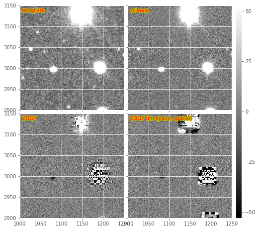
Figure 4 Subsections of a DECam Zogy image subtraction, including warped and PSF-matched template, science image, and the results of the “standard” and image-space versions of the Zogy algorithm.
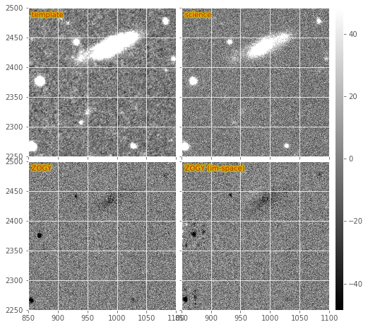
Figure 5 Subsections of the same DECam Zogy image subtraction as in Figure 4a.
Some additional notes about the fringing:
- The fringing might be a PSFex PSF-related artifact is consistent with the fact that I only see this fringing in real data where the PSFs have been measured (in the LSST stack, as I mentioned, the default is to use PSFex). When I originally ran the Zogy code on simulated images with smooth, double-Gaussian elliptical PSFs, I did not see such fringing. An example notebook where this is evident may be found here.
- This fringing was also observed by Tim Axelrod when using another Zogy implementation when a certain PSFex PSF configuration was used (pixel based? too small PSF dimensions? “It certainly is a result of bad parameters to psfex, and in particular the footprint size for determining the psf being way too big for this data.”). I include his example below in Figure 6, based upon DECam data. It appears to be an \(S_{corr}\) image (see Section 2.3, below). He was able to fix the fringing by changing the PSFEx parameters, but is unclear on the details.
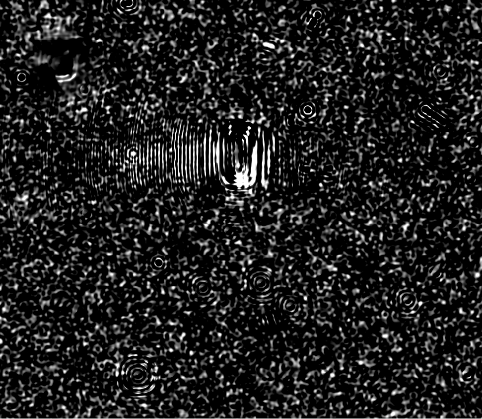
Figure 6 Example Zogy image with fringing from Tim Axelrod
Timing: The current implementation of Zogy takes roughly 26.6 seconds, or \(0.63\times\) as long (i.e., is \(\sim37\%\) faster) to run than the AL algorithm with decorrelation enabled. There has been limited attempt to date to optimize the Zogy algorithm, and some simple profiling is likely to highlight several bottlenecks.
Additional known issue: Zogy relies upon FFTs of the PSFs of both
input images. If those PSFs are not the same dimension, then one of them
needs to be padded or trimmed. We also need to ensure that the PSFs are
centered correctly, and centered at the same pixel coordinate. There is
much code in lsst.ip.diffim.zogy for making these corrections, yet
sometimes the resulting Zogy diffim has 1-pixel offsets from expected. I
have not yet been able to fix this in all cases, and it is not clear why
for some images this becomes an issue, while for others it is not.
2.1. Variants (image-space convolutions)
The convolutions in Zogy may be performed in image (real)-space rather
than in frequency space. This is beneficial in the LSST stack as then
the convolutions may be performed using the afw framework, which
accounts for masks and propagates the convolutions through to the
variance and mask planes of the exposures. The image-space convolution
Zogy images are shown in the bottom-right of Figure 4
and Figure 5. Because the convolution kernel is
spatially constrained, we see that the artifacts evident in the
“standard” Zogy implementation (bottom left of those figures) are also
spatially constrained. However, it is also evident that echo-like
artifacts are also generated in the image-space version which can be
severe surrounding the brightest stars. These artifacts lead to a
greater number of false positive detections (472 vs. 257 before merging
of positive and negative sources into a single footprint; 227 vs. 221
after).
Efforts were made to ensure that masks and variance planes are correctly
handled in the “pure” Fourier-space version of the algorithm, such that
the concerns about using afw for convolutions and handling
masks/variance correctly should be less of a concern.
Timing: The run-time of the image-space version of Zogy is \(\sim55.4\) seconds, or nearly \(2.1\times\) as long as the “pure” Fourier-space version. There are certainly some optimizations to be made if this path is pursued.
2.3. The ZOGY \(S_{corr}\) image
The Zogy manuscript describes the derivation of the “likelihood” image,
which they call \(S_{corr}\), because it may be corrected for
various terms such as astrometric errors/scintillation. This image is
analogous to the pre-convolved, decorrelated AL diffim in that it is
already pre-match-filtered with its own PSF, and thus may simply be
thresholded for detection. The Zogy code in ip_diffim has the option
of computing this image. Because of its similarity to the
pre-convolution option in AL, it is enabled in the
imageDifference.py command-line script by setting the config option
makeDiffim.doPreConvolve to True. We show an example
\(S_{corr}\) image in the bottom-right of Figure 7,
which may be compared with the AL version (non-decorrelated) on the
bottom-left of Figure 7 and both decorrelated and
non-decorrelated versions of AL at the bottom of Figure
3. The \(S_{corr}\) image again shows (what I believe
to be) the effect of inaccurate relative calibration between the two
input images.
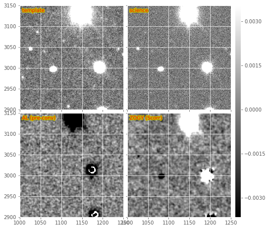
Figure 7 Subsections of a DECam Zogy image subtraction, including warped and PSF-matched template, science image, and the results of pre-convolved AL subtraction, and the Zogy \(S_{corr}\) likelihood image.
Timing: The computation of the Zogy \(S_{corr}\) image is roughly 10 to 20% slower than computing the standard Zogy diffim, depending upon whether the spatially varying options are enabled or not.
2.4. Issues, unimplemented aspects, artifacts
3. Spatial variations via ImageMapReduce
The calculations underlying both AL decorrelation and Zogy depend upon
factors with vary spatially across both input images, such as
PSF-matching kernel (AL) PSFs of both images (Zogy), and noise in both
images (AL and Zogy). Both algorithms also involve computing FFTs of
kernels or images, which cannot intrinsically include the spatially
varying components. Therefore, to capture these spatial variations, I
developed a flexible framework which “chops” the images into sub-images,
performs a given algorithm on those sub-images, and then “re-stitches”
the resulting modified sub-images back into a single exposure. This has
an analogy with the map-reduce algorithm, so it is called the
imageMapReduce framework, implemented in the submodule
lsst.ip.diffim.imageMapReduce.
3.1. imageMapReduce: Implementation details
The imageMapReduce framework may be visualized via the following
schematic (Figure 8). The ImageMapReduceTask chops
up the input Exposure into subExposures, which are then processed by
the ImageMapper. The modified subExposures are stitched back
together by the ImageReducer into a new Exposure.
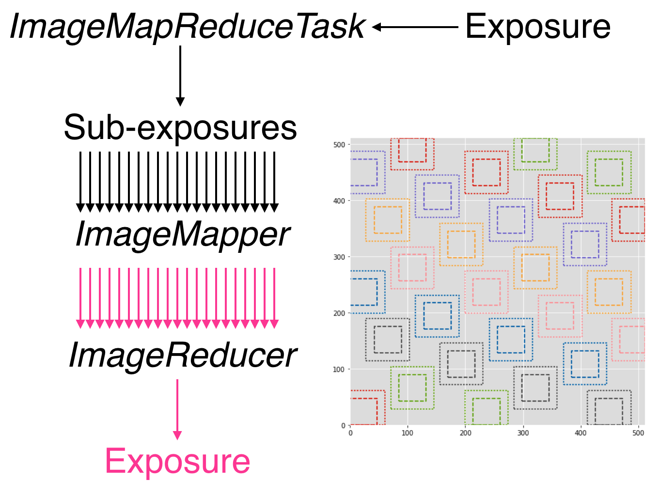
Figure 8 Schematic of the imageMapReduce framework for performing
spatially-varying calculations on one or more exposures. The inset
shows an example grid. Only every fifth grid element is drawn, for
clarity.
The ImageMapReduceTask accepts a set of configuration parameters
that specify how the grid is constructed (grid element size and
spacings). The grid specification is flexible so that it may contain
arbitrary overlapping regions between grid elements, and be of arbitrary
dimensions. The dimensions may also be specified in units of the FWHM of
the PSF of the input Exposure. An important detail is that one may
also specify an “expanded border” region for each grid element. If this
is done, then two subExposures are passed to the mapper subtask (see
below). An example grid is shown in the inset of Figure
7, including the “expanded” sub-regions in the dotted
lines.
The ImageMapReduceTask also accepts configuration parameters that
specify the mapper and reducer subtasks. The
ImageMapReduceTask then chops up the input Exposure and passes
those subExposures independently to the run method of its mapper
subtask. The mapper subtask is a subclass of ImageMapper, and
its run method performs the calculations on the subExposure,
returning a modified subExposure (optionally with a modified PSF), along
with other metadata. (It may optionally return something other than an
exposure, e.g. a float, which can be useful for, for example, computing
statistics or doing other measurements on a grid across the input
Exposure.) If the “expanded border” is specified (as is needed by both
AL decorrelation and Zogy) then two subExposures are passed to the
mapper‘s run method. The calculations are to be computed on the
expanded subExposure, and then the sub-image of the expanded subExposure
corresponding to the original grid element size is returned. This allows
operations such as convolutions or FFTs to be performed on the larger
image and the resulting invalid pixels at the borders are cut away
before passing the valid subExposure back to the reducer (see the
inset of Figure 8).
The returned, modified subExposures are then stitched together by the
reducer subtask into a final output Exposure, averaging the
overlapping regions (by default).
In order to perform spatially-varying AL decorrelation or Zogy, one
simply needs to subclass the ImageMapper task and the
ImageMapReduceConfig configuration class, and configure the
mapper parameter in that new config to point to this new subclass.
Known issues: The use of ImageMapReduce for spatially-varying
computations slows down the given computation (AL decorrelation or Zogy)
considerably. This is unsurprising, due to two extra sets of
calculations which are performed in the spatially-varying case: (1)
extra kernels are computed for each subImage; (2) multiple copies of
each exposure are made (both in pieces for the processing, and in one
final exposure when they are stitched together); and (3) extra image
area is processed due to overlapping regions of expanded subImages. Not
to mention the additional operations of splitting, and then re-combining
the subImages into a final exposure. This could be optimized by altering
the grid geometry. The default grid geometry splits the
\(\sim 1,024 x 2,048\) DECam CCD exposure into 1,128 subImages, and
given the expanded subImages, \(\sim 5\%\) more image is processed.
The prior (1,128 subImages) is probably overkill given the degree of
spatial variation that needs to be captured.
We also note that the construction of the grid itself is straightforward but may be brittle for certain image dimensions. The requirement of adjusting grid geometry for the given image dimensions should be addressed.
3.1.1. imageMapReduce: AL decorrelation
The spatially varying AL decorrelation is implemented in the
lsst.ip.diffim.imageDecorrelation submodule via the
DecorrelateALKernelMapper subclass of ImageMapper and the
corresponding DecorrelateALKernelMapReduceConfig subclass of
ImageMapReduceConfig. Then the DecorrelateALKernelSpatialTask
pipe task wraps the construction of the ImageMapReduceTask and
setting it up to use the DecorrelateALKernelMapper as its
mapper. It is this task (the DecorrelateALKernelSpatialTask)
that is called from the makeDiffim task.
Timing: The AL with the spatially-varying decorrelation takes 108.0
seconds with the default grid geometry configuration, or
\(2.4\times\) longer than the non-spatially-varying version. The
reason for this is due to the fact that (1) many more decorrelation
kernels are computed (276 of them), and (2) more area is convolved
(\(\sim 6.5\%\) more, due to overlapping grid elements) with the
imageMapReduced variant. See the Known issues subsection above
for more on this.
3.1.2. imageMapReduce: Zogy
The spatially varying AL decorrelation is implemented in the
lsst.ip.diffim.imageDecorrelation submodule via the ZogyMapper
subclass of ImageMapper and the corresponding
ZogyMapReduceConfig subclass of ImageMapReduceConfig. Then the
ZogyImagePsfMatchTask pipe task wraps the construction of the
ImageMapReduceTask and setting it up to use the
DecorrelateALKernelMapper as its mapper. It is this task (the
DecorrelateALKernelSpatialTask) is called from the makeDiffim
task.
Timing: The spatially-varying Zogy implementation takes \(\sim 43.0\) seconds, or \(\sim 1.5\times\) longer than the non-spatially-varying version. The reasons for this is unclear, except (as mentioned above) with the spatially-varying variant, the Zogy procedure is actually performed on significantly more image area (about 10% more) due to the necessity of overlapping grid elements. It is quite possible that the grid configuration could be modified to optimize this and bring down computation time; this has not been thoroughly investigated.
3.2. imageMapReduce: construction of new PSFs
Since the PSFs of image subtractions constructed via spatially-varying
computations are themselves expected to vary, we need to attach a new
PSF to the new exposures that contain that spatially-varying
information. A natural choice was to use a
lsst.meas.algorithms.CoaddPsf, which constructs, as it sounds, a
spatially-varying PSF by averaging PSFs from images which contributed to
various regions of a coadd. Since an Exposure constructed by
imageMapReduce is essentially a coadd, this seemed like a simple and
natural choice. It however has several disadvantages.
3.2.1. CoaddPsf issues
First, there will be slight discontinuities in PSF from one subregion to
the next. If the PSF is smoothly-varying, this should not be an issue,
but if a star falls on the edges of such a boundary, this could be a
problem. The degree or extent of this issue has yet to be explored. An
alternative is to construct a smoothly varying PSF fitted or
interpolated from the PSFs at the center of each grid element, e.g.
using lsst.meas.algorithms.PcaPsf.
Second, there is a significant issue with the speed of measurement. The
process of “finding” the correct PSF to use for a given region of an
image slows down any use of the CoaddPsf for spatially-varying
information. Detection uses a single PSF computed from the center of the
exposure, and thus is not slowed down, but measurement is slowed down
immensely in this case. This can (and should) be fixed, as above, by
using a smoothly-varying PSF subclass that was written for speed, such
as PcaPsf.
4. Dipole fitting complications
As described in DMTN-007, the measurement of dipoles was improved by incorporating “prior” information from the PSF-matched, warped template (we’ll call that \(T\)) and the science image (\(S\)) to constrain the dipole fitting, as well as the data from the image subtraction (\(D\)) itself. At the time it was assumed that AL would be used and decorrelation and/or Zogy were not yet invented. Thus, we used the (still correlated) warped and PSF-matched version of the template \(T'\) as input to the fitting algorithm. In fact, since we had all of the information, we passed \(T'\), \(S\), and \(D\) all to the dipole fitting algorithm.
AL decorrelation adds a complication that including the correlated warped PSF-matched template \(T'\) is not technically correct, since \(D\) is no longer equal to the decorrelated image subtraction (we’ll call that \(D'\)) minus \(T'\):
Instead, \(D'\) now equals \(S\) minus a decorrelated version of \(T\) (let’s call that \(T'\)), which we have not computed. However, we can compute
and then use the combination of \(T'\), \(S\), and \(D'\) for dipole fitting. Another complication arises that the PSF of \(T'\) has not been computed; however we will assume that it suffices to use the PSF of \(S\) (to which \(T\) has been PSF-matched).
This will not work for Zogy, however, since the template and science image are each convolved with a non-PSF-like kernel, which leads to them individually looking quite odd – but that oddness “cancels” when the images are finally subtracted in the end. In principle, we could simply feed the original science and warped (non-psf-matched) template to the dipole fitting code, as all they are really used for are to constrain the dipole lobe centroids. However, that will involve some modification of the dipole fitting code so that it can use three different PSFs – the template PSF for one lobe, the science image PSF for the other lobe, and the diffim PSF for the joint dipole fit. This would not be dificult; it has simply not been done.
5. Photometry
In DM-8796 I reviewed the photometry of diaSources recovered in simulated images using the various algorithms described above. Several issues were discovered. Note that all of these issues were discovered on simulated images and thus are not related to the issues discussed above associated with PSFex-measured PSFs. I will not rehash the details of those here, but will instead simply paste a slightly-edited copy of the summary here:
SNRs and forced photometry were assessed for all 4 flavors of diffim tested (Flavors: A&L, A&L(decorrelated), ZOGY(fully Fourier space), ZOGY(convolutions in image space). The forced photometry SNRs on diffims for all 4 flavors matched the expectation for the input PSFs and fluxes. These tests led to discovery of issues (bugs) with both ZOGY and A&L diffim decorrelation. The issues found and corrected included 1-pixel offsets in convolution kernels (and resulting PSFs). There are still three known issues with ZOGY and/or AL(decorr) that have yet to be solved, but these will be addressed in four tickets as determined to be necessary. These four issues and their corresponding new tickets are:
- DM-9442: ZOGY seems to have better performance than A&L(decorr) (better true-positive rate, similar rate of false positives). Part of this may be the windowing issue (losing detections in convolution window around image edge) but I tried to prevent any transients from being placed near edges and still seeing this effect a bit (~10% difference).
– Tested - could be misalignment of PSF. TRY: re-run with bigger matching radius (this is not the problem) – Tested - could be issue with ALdecorr PSF. TRY: compare ALdecorr PSF with ZOGY psf (PSFs are slightly different) – Tested - different PSFs are related to imperfect PSF matching. Tried other parameters for basis (e.g. make them somewhat smaller) which improved the AL result slightly.
- DM-9443: ZOGY(image space) has issues (artifacts) but only with measured PSFs, leading to fewer detections, more false positives. This is in comparison to ZOGY performed fully in Fourier space.
– This seems to be related to padding of the kernels. I fixed the padding (removed the “unpadding” step) and things improved a lot. Doing that and increasing the padSize removes much of the artifacts but increases the width of the invalid convolution “window” around the edges of the image. – TODO: investigate tradeoff between padding of PSF for ZOGY (image-space) vs. artifacts on real data.
- DM-9444: ZOGY (both kinds) has poorer performance when template is not noisy but only with measured PSFs, leading to fewer detections, more false positives
– TESTED - try with re-measuring science img PSF but not template PSF (no improvement)
- DM-9445: ZOGY S_corr is underperforming. This appears to be a regression. Likely due to the fact that I changed how the variance is computed for the Fourier-only-based ZOGY. But it could also just be a detection issue (detection for all other methods was changed to use pixel_stdev and positive only, but not changed for SZOGY).
5. Appendix
5.1. Summary of known issues with AL decorrelation and Zogy
While I described at various points above the known issues with the current LSST implementations of AL decorrelation and/or Zogy, here is a simple overview/summary of those known issues, including (if they have been made) their related tickets. It should be added that since the Zogy code has only recently been added to the LSST stack and minimally applied to actual data, there could be other issues that are not yet known.
- DM-11993: Occasional issues with AL decorrelation, which lead to strange fringing/periodic wave-like artifacts. The cause is unknown and the situation is not completely understood; probably related to the shape/structure of the PSF matching kernel. Note that if the term in the denominator of the expression for \(\psi(k)\) is too close to zero, it will lead to large values in the kernel, which could lead to strange aliasing artifacts in the resulting decorrelated diffim. This is a rare occurrence, and I have only seen it recently on poorly-calibrated WISE images.
- DM-11994: AL decorrelation when pre-convolution is enabled has similar issues to (1.) above but more frequent. Probably also due to similar causes which are exacerbated by the inclusion of a noisy PSF in the decorrelation kernel term.
- DM-11991: Zogy suffers if there is inaccurate relative calibration between the two images. This issue can be seen in nearly all of the Zogy images shown in this document. Not clear how frequently this occurs. This can be fixed by fitting for the relative calibration and setting them as the Fr and Fn parameters for Zogy, or else ensuring that the LSST stack calibration is accurate. Another possibility is that the images are not being loaded for Zogy correctly or that a (already measured?) flux calibration should be applied to the pixels in the images before running Zogy.
- DM-11990: Occasionally seen with both Zogy and AL Decorrelation: depending upon the dimensions of PSFs/kernels/input images, the resulting Zogy diffim or decorrelated diffim can have an erroneous 1-pixel offset (shift). Several attempts have been made to fix this but it still occurs on occasion.
- DM-10805,
DM-9443: Fringing in
Zogy diffim (see Figure 4b). Possibly related to the
use of certain PSFex parameters in computing the PSFs for the two
input images (as suggested by Tim Axelrod; see above). Another
consideration could be related to the interpolation used for template
warping; this has not been investigated. The spatial extent of these
fringing artifacts is limited by ensuring that PSFs don’t decrease
below a certain level (thus eliminating very small or negative
numbers in the Zogy diffim expression), and/or increasing the size of
the
ImageMapReducegrid elements. - DM-9443: Artifacts in
the Zogy diffim when convolutions are computed in image (real) space
(again, see Figure 4b). Could have the same causes
as the fringing in the Fourier-based Zogy diffim. Possible additional
fixes could include increasing the padding of the PSFs, and/or
increasing the size of the
ImageMapReducegrid elements. - DM-11995: The
ImageMapReduceframework for computing Zogy or AL decorrelation in a spatially-varying manner across an image could benefit from an improved method to compute the grid geometry for any given exposure/PSF dimensions that is less brittle and could probably speed up the operation significantly. - DM-10806: PSFs for
exposures generated by the
ImageMapReduceframework are currentlyCoaddPsfs, which are fine for detection but very slow for measurement. This needs to be changed, orCoaddPsf(or a subclass thereof) needs to be optimized. See the relevant section. - DM-6894: The new
DipoleFittingscheme does not work for Zogy images, however an alternative is described in Section 4, but this will complicate the code such that a different scheme is used whether the diffim was computed via Alard & Lupton or ZOGY.
5.2. Summary of diffim algorithm timings
At the end of each subsection above, I listed the run-time timings of each algorithm/component. Below is a summary table of those findings. These are for runs on a single DECam CCD exposure, with a single CCD exposure used as the template, using a single CPU on a Macbook Pro with a 2.5 GHz Intel Core i7.
| Alg. | Spatial? | Pre-conv.? | Time (sec.) | |
|---|---|---|---|---|
| AL | No | 31.8 | ||
| AL + decorr. | No | No | 42.5 | |
| AL + decorr. | Yes | No | 108.0 | |
| Zogy | No | No | 26.6 | |
| Zogy | Yes | No | 43.0 | |
| Zogy (im-space) | No | No | 55.4 | |
| Zogy (im-space) | Yes | No | 246.3 | |
| AL | Yes | 55.8 | ||
| AL + decorr. | No | Yes | 67.8 | |
| AL + decorr. | Yes | Yes | 138.4 | |
| Zogy | No | Yes | 32.7 | |
| Zogy | Yes | Yes | 62.7 |
5.2.1. Random thoughts and notes for improving algorithm efficiency
- Currently the Zogy implementation uses
numpy.fft.fft2and related for computing 2-D FFTs. It should be noted that thescipy.fftpackimplementation has been found to be slightly faster, while thefftwlibrary (with python bindings pyFFTW can be significantly faster. Moreover, there is little effort made to pad matrices to \(2^n\) dimensions, which if done can also speed up the Fourier transforms. Little effort has been made to investigate this further since at this point it is not clear how much the FFTs bottleneck the procedure. - The primary bottleneck that appears to be slowing down the AL
decorrelation is the convolution of the diffim with the decorrelation
kernel. This is currently performed by
afwcode and takes \(\sim 10\) seconds for the single DECam exposure. It is not clear if the decorrelation kernel is not properly optimized for this convolution, or what else might be the cause for this slowdown.
5.4. Commands for running image subtraction in various modes
Example output from the various runs of the image subtraction pipeline on a single pair of DECam exposures is shown in the notebook attached to this DMTN’s repository. Scripts were used to perform these runs, and they have been saved in the DM-3704 branch of ip_diffim and of pipe_tasks. The data itself have been uploaded to the dmtn-061-data repository. I now summarize these command-line configurations below. I also include the redirected output text files in this repo as well.
Configuration file
diffimConfig.pyforimageDifference.py:config.makeDiffim.doWriteSubtractedExp=True config.makeDiffim.doWriteMatchedExp=True config.makeDiffim.doDecorrelation=True config.makeDiffim.subtract='al' config.makeDiffim.subtract['zogy'].zogyConfig.inImageSpace=False from lsst.ip.diffim.getTemplate import GetCalexpAsTemplateTask config.getTemplate.retarget(GetCalexpAsTemplateTask)
Run AL with and without decorrelation, (and decorrelation both constant and spatially-varying):
imageDifference.py calexpDir_b1631 --output decamDirTest_AL \
          --id visit=289820 ccdnum=11 --templateId visit=288976 \
          --configfile diffimConfig.py --config makeDiffim.doDecorrelation=False >& \
            output_AL.txt

imageDifference.py calexpDir_b1631 --output decamDirTest_ALDec_noSpatial \
          --id visit=289820 ccdnum=11 --templateId visit=288976 \
          --configfile diffimConfig.py >& output_ALDec_noSpatial.txt

imageDifference.py calexpDir_b1631 --output decamDirTest_ALDec_yesSpatial \
          --id visit=289820 ccdnum=11 --templateId visit=288976 \
          --configfile diffimConfig.py --config makeDiffim.doSpatiallyVarying=True >& \                 output_ALDec_yesSpatial.txt
- Run Zogy (both constant and spatially-varing) and try both in Fourier and real space:
imageDifference.py calexpDir_b1631 --output decamDirTest_Zogy_noSpatial \
          --id visit=289820 ccdnum=11 --templateId visit=288976 \
          --configfile diffimConfig.py --config makeDiffim.subtract='zogy' >& \
                output_Zogy_noSpatial.txt

imageDifference.py calexpDir_b1631 --output decamDirTest_Zogy_yesSpatial \
          --id visit=289820 ccdnum=11 --templateId visit=288976 \
          --configfile diffimConfig.py --config makeDiffim.subtract='zogy' \
          --config makeDiffim.doSpatiallyVarying=True >& output_Zogy_yesSpatial.txt

# replace 'inImageSpace=False' with 'inImageSpace=True' in diffimconfig.py
imageDifference.py calexpDir_b1631 --output decamDirTest_ZogyImSpace_noSpatial \
            --id visit=289820 ccdnum=11 --templateId visit=288976 \
            --configfile diffimConfig.py --config makeDiffim.subtract='zogy' \
                >& output_ZogyImSpace_noSpatial.txt

# replace 'inImageSpace=False' with 'inImageSpace=True' in diffimconfig.py
imageDifference.py calexpDir_b1631 --output decamDirTest_ZogyImSpace_yesSpatial \
            --id visit=289820 ccdnum=11 --templateId visit=288976 \
            --configfile diffimConfig.py --config makeDiffim.subtract='zogy' \
            --config makeDiffim.doSpatiallyVarying=True >& \                output_ZogyImSpace_yesSpatial.txt
- As mentioned above, run AL and Zogy with
makeDiffim.doPreConvolve=Trueto create pre-filtered diffim (\(S_{corr}\) in Zogy parlance). Note that the Ids for thevisitandtemplateIdwere swapped in this case. - Finally, all of the timings listed above were measured using just the
makeDiffim.pycommand-line task, which performs image subtraction but not detection and measurement. This requires a slightly different config,makeDiffimConfig.py:
config.doWriteSubtractedExp=True
config.doWriteMatchedExp=True
config.doDecorrelation=True
config.subtract='al'
config.subtract['zogy'].zogyConfig.inImageSpace=False
from lsst.ip.diffim.getTemplate import GetCalexpAsTemplateTask
config.getTemplate.retarget(GetCalexpAsTemplateTask)
And below are the commands used (prior to each run, rm -r DELETEME
was performed):
time makeDiffim.py calexpDir_b1631 --output DELETEME --id visit=289820 ccdnum=11 \
    --templateId visit=288976 --configfile makeDiffimConfig.py \
    --config doDecorrelation=False

time makeDiffim.py calexpDir_b1631 --output DELETEME --id visit=289820 ccdnum=11 \
    --templateId visit=288976 --configfile makeDiffimConfig.py \
    --config doDecorrelation=True

time makeDiffim.py calexpDir_b1631 --output DELETEME --id visit=289820 ccdnum=11 \
    --templateId visit=288976 --configfile makeDiffimConfig.py \
    --config doDecorrelation=True --config doSpatiallyVarying=True

time makeDiffim.py calexpDir_b1631 --output DELETEME --id visit=289820 ccdnum=11 \
    --templateId visit=288976 --configfile makeDiffimConfig.py --config subtract=zogy

time makeDiffim.py calexpDir_b1631 --output DELETEME --id visit=289820 ccdnum=11 \
    --templateId visit=288976 --configfile makeDiffimConfig.py --config subtract=zogy \
    --config doSpatiallyVarying=True

rpl -q 'inImageSpace=False' 'inImageSpace=True' makeDiffimConfig.py
time makeDiffim.py calexpDir_b1631 --output DELETEME --id visit=289820 ccdnum=11 \
    --templateId visit=288976 --configfile makeDiffimConfig.py --config subtract=zogy
rpl -q 'inImageSpace=True' 'inImageSpace=False' makeDiffimConfig.py

time makeDiffim.py calexpDir_b1631 --output DELETEME --id visit=288976 ccdnum=11 \
    --templateId visit=289820 --configfile makeDiffimConfig.py \
    --config doDecorrelation=False --config doPreConvolve=True

time makeDiffim.py calexpDir_b1631 --output DELETEME --id visit=288976 ccdnum=11 \
    --templateId visit=289820 --configfile makeDiffimConfig.py \
    --config doDecorrelation=True --config doPreConvolve=True